Geophysical methods for soil applications
Abstract
Traditional methods to assess soil properties or monitor soil processes typically rely on point data. They often fail to represent the heterogeneity of soil. Airborne remote sensing techniques allowed us to measure proxies for soil properties or variables at regional scale, but often covering only the first few centimeters of soil. Ground-based geophyscial methods can fill in the gap between these two scales. They primarily observe variations in the thermal, electrical, magnetic, electromagnetic and/or seismic properties of the subsurface to map its characteristics or to monitor dynamic changes and can yield 2- or 3-D quantitative information on soil properties or processes. Geophysical methods have been applied in various soil-related research fields: from soil mapping and precision agriculture, to geotechnical engineering and soil remediation and to archeology and forensic investigation. This chapter briefly introduces the ground-based geophysical techniques appropriate for soil applications.
Keywords
geophysics, soil management, non-invasive, electrical resistivity tomography, ground-penetrating radar, distributed temperature sensing, seismics, nuclear magnetic resonance, magnetometry, induced polarization, electro-magnetic induction, inversion, pedophysical relationship
Key points
- Geophysical methods are key to bridge the gap between point measurements and remote sensing techniques for soil applications.
- This chapter introduces the ground-based geophysical techniques relevant for soil applications, commonly used equipment and limitations of each technique
- The use of geophysical techniques for soil applications ranges from soil mapping and precision agriculture, through geotechnical engineering and soil remediation and to archeology and forensic investigation.
- We discuss critical data processing steps such as inversion and pedophysical relationships.
Introduction
The soil plays a crucial role in the redistribution of energy, water and solutes in terrestrial systems. Relevant scales range from the single pore and the soil-root interface through the field scale to encompass the entire globe. The multi-scale heterogeneity of soils presents a challenge to the representation of processes over different scales and to the parameterization of corresponding models. Traditional observation methods for soil processes often rely on (a network of) point data from manual sampling or sensors that capture states and attributes of soil system functioning. These point data often fail to capture the heterogeneity of soil properties at larger scale. Over recent decades, airborne remote sensing techniques (from drones to satellites) generated proxies for near-surface soil properties at the regional scale (eg. SMOS, SMAP, Sentinel-1, Sentinel-2 campaigns). Nevertheless, those methods only interrogate the first few centimeters of the soil. In addition, the time-intervals between measurements and spatial resolution are rather coarse (days and 10-100s of meters, respectively). Ground-based geophysical methods can fill in the gap between local point measurements and remote sensing products Romero-Ruiz et al., 2018. Geophysical methods typically observe variations in the thermal, electrical, magnetic, electromagnetic or seismic properties of the subsurface to map its characteristics or to monitor dynamic changes. They can yield 2- or 3-D information on soil properties (e.g., texture or organic matter content) or state variables of interest (e.g., temperature, soil moisture, salinity) at centimeter or decimeter resolution.
This chapter briefly introduces key ground-based geophysical techniques relevant for soil applications, commonly used equipment and limitations of each technique. The use of unmanned aerial vehicle (UAVs) for geophysical surveys (e.g. EMI, GPR, magnetometry) or sensors mounted on towers (e.g. L-band radiometry, cosmic-ray neutron sensing) are not covered here, but is certainly also relevant for soil applications. Airborne GPR and EM are increasingly being used on UAVs as recently reviewed in Auken et al. (2017), for example.
Geophysical variables and pedo/petrophysical models
For a geophysical measurement, we register the response of the soil to a signal which is naturally present (e.g. gravity) or which is actively introduced by the observer (e.g. an electrical current). For soil applications, electromagnetic energy is most used, alongside acoustic waves and gravitational fields. In all cases, the observed change in voltage in the measurement device is related to the geophysical response. The most straightforward example of this process is the direct current (DC) resistivity method (Section %s), whereby a current I is introduced into the soil, after which the resultant potential difference (or voltage V) between pairs of electrodes is recorded with a voltmeter. The resistance of the recorded volume is then obtained through Ohm’s law. To translate the collection of signals (e.g. resistances) to a distribution of the geophysical property (e.g. the electrical resistivity distribution of the bulk soil), we then have to incorporate information on the measurement geometry, the physical processes taking place during the measurement and the nature of the soil in a process called ‘inversion’ (see Section %s).
Typically, the inferred geophysical properties are not the primary property of interest, but they are used as a proxy for a soil characteristic or state variable. Therefore, relationships are established between these properties of interest and the geophysical properties. Such relationships are called petrophysical or, in the field of soil science, pedophysical relationships Wunderlich et al., 2013. A pedophysical relationship expresses the influence of different soil properties and state variables on the geophysical property. Soil electrical resistivity is for example affected by, amongst others, pore water salinity, soil texture, porosity, temperature and soil moisture. Therefore, several sources of independent data or calibration data are necessary to develop pedophysical relationships. We give an overview of the geophysical methods, the properties measured and examples of the derived properties and states in Table 1. We redirect the reader to Binley & Slater (2020) for further details.
Table 1:Geophysical methods, their properties measured and examples of derived properties and states (adapted from Binley et al. (2015))
Geophysical Method | Common abbreviations | Geophysical Properties | Examples of Derived Properties and States |
|---|---|---|---|
Electrical resistivity tomography | ERT, ERI | Electrical conductivity | Water content, clay content, pore water conductivity |
Induced polarisation | IP, EIT | Electrical conductivity, chargeability | Water content, clay content, pore water conductivity, surface area, permeability |
Spectral induced polarisation | SIP | As above but with frequency dependence | Water content, clay content, pore water conductivity, surface area, permeability, geochemical transformations |
Self-potential | SP | Electrical sources, electrical conductivity | Water flux, permeability |
Electromagnetic induction | EMI, FDEM, TDEM | Electrical conductivity | Water content, clay content, salinity |
Magnetic susceptibility | Ferromagnetic iron oxide content, redox conditions | ||
Magnetometry | MAG | Magnetic suceptibility, Remanent magnetisation | Ferromagnetic iron oxide content, redox conditions. |
Ground penetrating radar | GPR | Permittivity | Water content, porosity, stratigraphy |
Seismic | Elastic moduli and bulk density | Lithology, ice content, cementation state, pore fluid substitution | |
Seismoelectrics | Electrical current density | Water content, permeability | |
Nuclear magnetic resonance | NMR | Proton density | Water content, permeability |
Gravity | Bulk density | Water content, porosity | |
Distributed temperature sensing | DTS | Temperature | Water content, thermal properties (conductivity and diffusivity) |
Applications of geophysical methods in soil science
During the past decade geophysical measurement and data processing techniques became more affordable and easier to deploy. As such, these instruments offered the potential to explore and monitor the spatio-temporal dynamics of soil. In their review on hydrogeophysics, Binley et al. (2015) pointed out the expanding range of applications: from ecosystem science and biogeochemistry to agronomy and soil mapping. Since then, the possibilities have only expanded. Civil and geotechnical engineering problems are increasingly addressed using geophysics, especially when the application is water-related. For example, ERT, GPR, and self-potential (SP), combined with high-precision leveling, are used to assess sinkhole risks Giampaolo et al., 2016 and several authors have used ERT to monitor landslide activity Perrone et al., 2014. Another common application is soil pollution and remediation monitoring in polluted sites (e.g. Day-Lewis et al. (2017)). The efficiency of geophysical techniques for soil remediation monitoring greatly depends on the nature of the pollution and how it results in specific electrical or magnetic signatures. Geophysical methods have become ubiquitous in archaeological practice and heritage management. The first applications started in the 1950s and 1960s Gaffney, 2008. Magnetometry instruments are the workhorse for archaeological prospecting, complemented with ground penetrating radar, direct-current resistivity and electromagnetic induction surveys. Archeological applications have also driven the deployment of geophysical instrument (arrays) geared at high sensitivity and sampling density Trinks et al., 2018. Geophysics is also used for forensic investigations. For example, Doro et al. (2022) used ERT to locate clandestine graves and monitor human decay within the subsurface.
Precision agriculture is one of the fastest growing soil-centered areas for adopting geophysical methods. Where EMI has been used for years as a qualitative soil mapping tool or for more detailed experimental design Rudolph et al., 2016, multi-geometry devices now allow for inversion of the apparent electrical conductivity, unlocking information of vertical heterogeneity in addition to horizontal patterns. Combination with machine learning techniques has resulted in new possibilities Brogi et al., 2021. RomeroRuiz et al. (2021) used seismics to locate areas suffering from chronic soil compaction. GPR has been used at several sites to locate tile drainage components Koganti et al., 2020. Also, the monitoring potential of EMI and ERT and its relationship with soil moisture has been extensively used Blanchy et al., 2020. Several researchers use geoelectrical methods to study the root water uptake of trees and crops and estimate the efficiency of applied irrigation patterns Vanella et al., 2020Garré et al., 2013. This has led to the application of EMI, and also ERT, in plant phenotyping through the assessment of soil moisture depletion Whalley et al., 2017. Previously, the phenotyping community struggled to incorporate environmental effects into its studies in field environments, especially for the below-ground' part of the plant. Geophysics offers a window into that ‘hidden half’. Figure 1 gives an overview of the field setup of different geophysical techniques covered in the chapter.
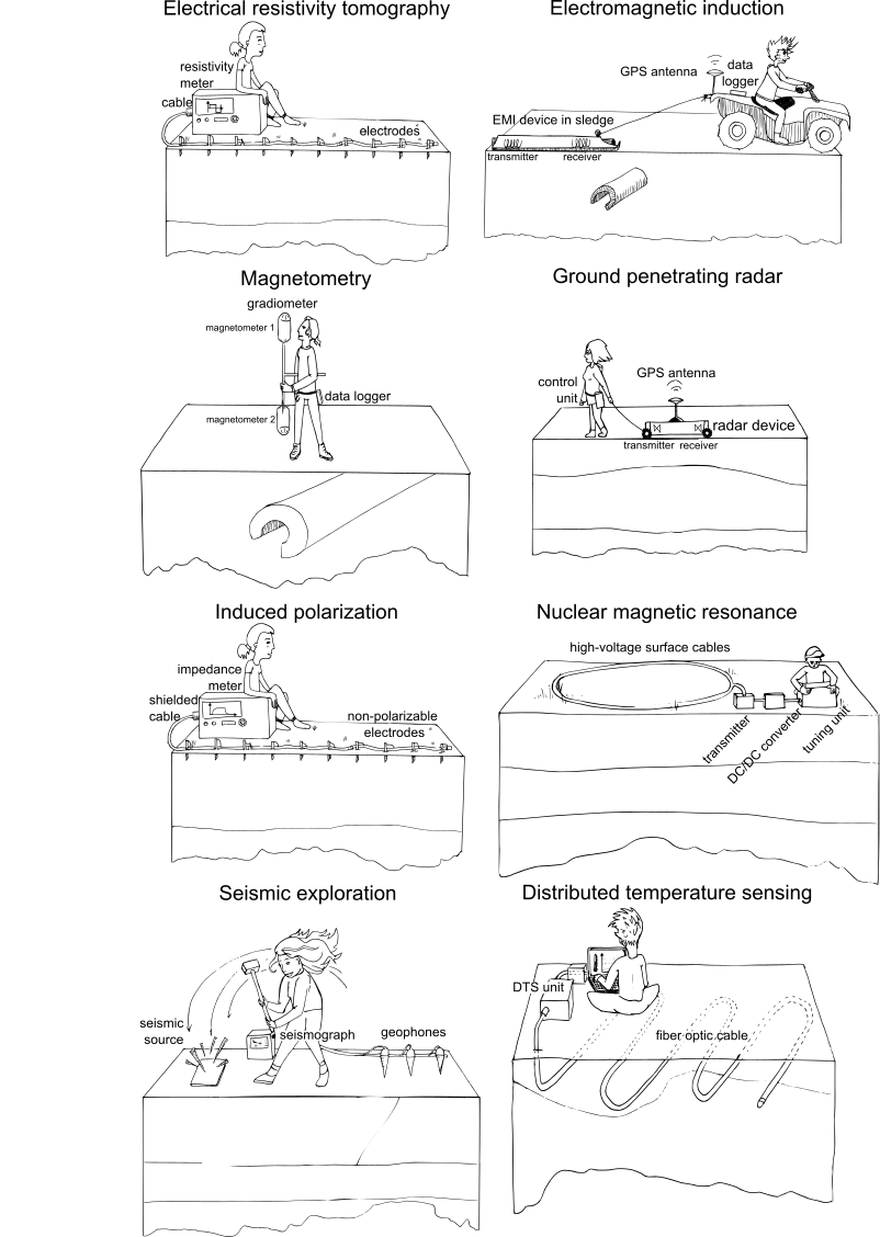
Figure 1:Overview of the field setup for the different geophysical techniques for soil applications covered in this chapter.
Electrical resistivity tomography (ERT)
Electrical Resistivity Tomography (ERT) is a technique, which infers the bulk electrical resistivity of the soil between electrodes. The bulk electrical resistivity corresponds to the combined resistivity of soil particles, pore water and air. A basic measurement system consists of four electrodes (A, B, M, N), a transmitting electrode pair and a receiving electrode pair. The transmitter electrode pair applies a quasi-direct(i.e rectangular DC current pulses or an AC current at low frequency to avoid polarization) current (I) to the ground using rectangular DC current pulses or an AC current at low frequency to avoid polarization of injection electrodes A and B. The receiver measures the voltage (V) between the potential electrodes M and N (see Figure 2). Resistivity meters then register a resistance (R) for each combination of four electrodes, based on Ohm’s law R = V/I. For a tomography, many different combinations of current and potential electrodes are used for injection and measurement. The electrodes can be inserted into the soil surface or at several depths as borehole electrodes or a combination of both.

Figure 2:Basic concept of electrical resistivity measurement of the subsurface
From the current, the voltage and a geometric configuration factor (k), the apparent electrical resistivity (ρa) is calculated. The geometric factor depends on the spatial arrangement of the four electrodes and the geometry of the measurement area (e.g. presence of topography). Resistance is an extrinsic property (i.e., depends on the way it is measured), whereas resistivity is an intrinsic property (i.e., depends only on the material in which the measurement is performed). We call the obtained resistivity “apparent”, because it represents the resistivity of a hypothetical, homogeneous medium, which would give the same resistance value for the applied electrode arrangement. The measured, apparent resistivity is a complex average of the resistivities of the various materials that the current encounters.
A soil-specific pedophysical relationship is necessary to derive any soil state variable or property from electrical resistivity measurements. A well-known electrical resistivity model is the empirical Waxman & Smits (1968) model that extends Archie’s Law Archie, 1942 to account for surface conduction. Apparent resistivity is also affected by temperature. Ma et al. (2010) gives an overview of temperature correction models.
Challenges and limitations
At the core of geoelectrical methods for application to soil is the assumption that the electrical conductivity map obtained of the subsurface can be translated into soil properties or state-variables via site-specific pedo-electrical relations calibrated with laboratory or field data. Common practice assumes spatially homogeneous relations, which neglects the impact of soil heterogeneity on those relations. This can cause significant errors in translating the electrical measurements to the hydraulic state variables Moreno, 2022. Standardized approaches to establish and upscale pedophysical relationships are, therefore, crucial to increase the accuracy of the method. Furthermore, the inversion remains a source of uncertainty, since an infinite number of electrical conductivity models fit the noisy geoelectrical data equally well (see Section %s).
Electromagnetic induction (EMI)
EMI uses low-frequency electromagnetic fields to investigate electrical and magnetic properties of the subsurface. For most soil applications, EMI measurements are performed in the frequency domain and described as frequency domain electromagnetics (FDEM). This means that the analysis of the signal is done with respect to frequency, rather than time. A magnetic field oscillating at a frequency between 1 - 100 kHz is generated by passing an alternating current through a transmitter coil (Tx, see Figure 3) that consists of a small wire loop Frischknecht et al., 1991. This primary field () induces eddy currents(Eddy currents (also called Foucault's currents) are loops of electrical current induced within conductors by a changing magnetic field in the conductor according to Faraday's law of induction) in conductive parts of the soil, which in turn generate a secondary magnetic field () that induces an oscillating current in the receiver coil (Rx). The size and shape of the subsurface volume that influences the observed current depends on the separation and respective orientation of transmitter versus receiver coil. For soil applications, coils are generally horizontally or vertically coplanar, or in a perpendicular orientation. One or more transmitter-receiver pairs are fixed in a rigid boom (so-called fixed-loop systems) with coil separations ranging from 0.20 m to 6.00 m. Although multi-frequency instruments are available (e.g., Won et al. (1996)), fixed-loop instruments used for soil applications operate at a single operating frequency, but integrate multiple transmitter-receiver pairs to enable geometrical depth sounding.

Figure 3:Diagram of the FDEM working principle, indicating the primary () and secondary () magnetic fields.
Evaluating the ratio of the secondary () to the primary magnetic field () at the receiver when both fields are out-of-phase or in-phase allows electromagnetic properties of the investigated volume to be derived. In low-conductive environments, the out-of-phase response is quasi-linearly related to the subsurface apparent conductivity McNeill, 1980. This approximate, but straightforward, relationship is only valid under certain conditions, requiring a sufficiently small Tx-Rx distance, operating frequency and subsurface conductivity Callegary et al., 2007. It is typically referred to as the low induction number approximation (LIN). Some instruments use multiple frequencies for different Tx-Rx distances to remain under this condition. When this condition is not met, e.g., in saline environments, the relationship becomes more complex and a full evaluation of Maxwell’s equations is needed to obtain reliable apparent conductivity values Hanssens et al., 2019. Commercially available instruments developed for soil applications usually output the out-of-phase response as apparent electrical conductivity () using the LIN approximation. Hence, they underestimate subsurface apparent electrical conductivity at higher conductivities and do not always offer access to the raw data.
In low-conductive environments (ca. <100 mS/m) the in-phase response informs on changes in soil magnetic susceptibility (). Although not widely used, current instrumentation allows reliable large-area mapping of soil susceptibility alongside apparent conductivity De Smedt et al., 2022. Relating the in-phase response to quantitative changes in subsurface magnetic susceptibility can be ambiguous due to complex spatial sensitivities and the influence of conductivity on this component. Nevertheless, recent advances show the potential of soil magnetic susceptibility modelling Klose et al., 2018Delefortrie et al., 2018.
Challenges and limitations
Although current FDEM instruments are increasingly well-calibrated, issues of absolute and relative signal calibration burden data interpretation. Offsets from absolute zero, i.e., resulting in a non-zero response when making air readings, mainly exacerbate quantitative interpretation of the in-phase response, while, particularly under the influence of temperature variations, drift with time introduces errors in all signal components, Hanssens et al., 2021. Accounting for these issues is required to allow reliable quantitative data interpretation. To this end, adaptive calibration Thiesson et al., 2014 and drift correction protocols Delefortrie et al., 2014 are available. Resolving these issues can aid exploiting the full potential of inversion methods geared towards 3D models of soil conductivity and magnetic susceptibility.
Magnetometry and magnetic soil mapping
Magnetometry is a passive method that measures ambient magnetic fields. The interplay between Earth’s magnetic field and magnetic materials in the subsurface lies at the heart of magnetometric prospecting Aspinall et al., 2008. Magnetic materials can be considered as magnetic dipoles that are magnetised by the influence of Earth’s magnetic field (see Figure 4). In addition, those materials can posses a residual magnetisation (remanence), which persists after an external magnetic field is removed and remains independent of weak magnetic fields Clark, 1997. This is common in anthropogenic materials, such as iron objects or clay bricks, that obtain remanence through the production process. At any location, the resulting total magnetic field can be measured and described by its intensity, and its directional components. Crucial in magnetometer surveying is accounting for the influence of diurnal variations in Earth’s magnetic field intensity, which are in the same order of magnitude of soil magnetic variations as natural and anthropogenic processes. To remediate this, stationary magnetometer measurements are conducted alongside roving measurements and subtracted from the survey data. Alternatively, magnetometers can be used in gradiometer mode, whereby two magnetometers are positioned at a fixed distance along the same axis. In such a configuration, the difference between the observations from both sensors is taken to remove diurnal variations, and provide more detailed insight into soil variations.

Figure 4:Diagram of the working principle of a magnetometer showing various instrument configurations (vertical gradiometer, whereby observations of the upper sensor are subtracted from those from the bottom sensor) and inclusion of a stationary base station for recording diurnal geomagnetic variations).
Two main types of magnetometers are in use: (i) total field magnetometers measuring the total magnetic field intensity and providing a scalar measurement (e.g., alkali-vapour (mainly caesium-vapour) magnetometers), and (ii) magnetometers recording a vector component (e.g., fluxgate instruments). The latter type is often configured in gradiometer mode as standard, i.e., as fluxgate gradiometers. More detailed discussions of the principles of magnetometry can be found in Aspinall et al. (2008) and Everett (2013). Apart from dominating the use of geophysical methods in archaeology Fassbinder, 2015, and use in unexploded ordnance detection Won, 1995, magnetometry is rarely deployed in soil applications. Pilot studies, however, have shown that even the weakly magnetic signal rendered by iron oxides in soils can be used to detect influence of soil tillage Mathé & Lévêque, 2003, whereas clay brick drainage pipes are straightforward magnetic targets due to their strong magnetic remanence Rogers et al., 2006.
Alongside magnetometry, other methods enable magnetic soil mapping by targeting the induced magnetisation, or magnetic susceptibilty, directly. Complementing the potential of FDEM instruments, dedicated susceptibility meters (e.g., Bartington MS2 Dearing, 1994 are used to map the magnetic signal of topsoils in pollution (e.g., Declercq et al. (2019)) or ecological studies (e.g., Grimley et al. (2008)). Such instruments, consisting of inductor-capacitor circuits operating through principles of electromagnetic induction, only offer small depths of investigation that are limited to the upper centimeters below the surface Lecoanet et al., 1999. Downhole logging configurations, however, can be deployed to gain better insight into vertical magnetic variations (e.g., as in Declercq et al. (2019)).
Challenges and limitations
The inherent relationship between the soil magnetic signal and its mineralogical composition, as well as its independence from short-term moisture dynamics, presents good opportunities for soil applications. Broadly described, the soil magnetic signal is influenced by pedogenic processes (such as weathering, reduction and oxidation of iron-bearing minerals) and anthropogenic processes (e.g, the heating of soil or the input of detrital materials such as magnetic particulate matter), which both primarily occur in the upper soil layer, as well as the lithology of the parent material (e.g., weathering of igneous bedrock). A comprehensive overview discussion on pathways to soil magnetism is provided by Jordanova (2017).
Magnetometer surveys have potential to study soil erosion Jordanova et al., 2014, redox variations Grimley et al., 2008, or as an indicator for the spatial distribution of soil nutrients Miroshnychenko et al., 2021. Here, combined use of adaptive instrumentation, for instance FDEM instruments operating at different frequencies Shirzaditabar & Heck, 2022, or the joint deployment and inversion of FDEM and magnetometry instrumentation can provide a more robust basis for field applications of magnetic soil mapping. Nevertheless, more work is needed to consolidate the fundamental framework for relating magnetic observations to investigated aspects of soil functioning across different soil types Jordanova, 2017.
Ground penetrating radar (GPR)
Ground penetrating radar (GPR) uses electromagnetic fields in the mega-to-gigahertz (MHz - GHz) range to characterize the soil. Compared to EMI, these higher frequencies put GPR in the propagation regime, whereby the emitted fields behave as waves that propagate, reflect and refract in the media they travel through. Acquisition of GPR data can be done very rapidly (see Figure 1) and, due to its wave-based nature, this method provides a much higher vertical (depending on soil properties and the source frequency) and horizontal resolution than other geophysical methods (e.g., ERT or EMI). For this reason, the GPR method is one of the most widely used geophysical methods in soil sciences and near surface surveying Knight, 2001Annan, 2005. GPR instruments are composed of a transmitting (Tx) and a receiving (Rx) antenna (see Figure 5). The former sends an electromagnetic wave into ground, after which the receiver records the reflections of the emitted wave as it travels through the soil. The velocity of the wave is determined by the soil dielectric permittivity (). When the electromagnetic wave encounters a change in permittivity, part of the energy of the wave is reflected on the interface, while the remaining energy is transmitted or refracted. Recording these reflections at the receiver provides information on the structure of the subsurface (Figure 5). These reflections are recorded in function of time, resulting in a so-called GPR-trace at each measurement location, traces can be aggregated in transects (radargram) or 3D volume. Several processing steps are needed to allow reliable interpretation of GPR data: the removal of interfering frequencies (e.g, background removal and ‘dewow’), converting wave traveltimes to depth (velocity analysis and migration) and adjusting signal gain (to compensate, for instance, for energy loss with depth). An overview of standard GPR processing steps is given by Cassidy (2009).

Figure 5:Diagram of the GPR working principle. On the right, a GPR trace is shown as would be obtained from the received reflections shown in the diagram.
The dielectric permittivity can be linked to other soil characteristics such as soil moisture content. This relationship has been widely used for Time-Domain Reflectometry (TDR) soil moisture sensors. Similarly, GPR has been used to map soil moisture by measuring the direct (not reflected) wave (Figure 5) that travels along the ground surface Algeo et al., 2016 or using air-launched methods Wu et al., 2019. However, these methods usually only assess the soil moisture of the upper layer (few centimeters). Transmission GPR can also be used to measure larger volume by using the wave speeds between boreholes Klotzsche et al., 2019. Huisman et al. (2003) provided a review of the use of GPR for soil moisture estimation. GPR can also be used to locate the depth of soil horizons with different soil texture and associated water retention properties (thus producing abrupt vertical changes in water content) André et al., 2012. In water-saturated conditions, GPR methods may help in locating zones with different porosities (i.e., different water content) or fractures, both associated with zones of increased permeability. Due to its simplicity, the empirical Topp’s equation Topp et al., 1980 is typically used to relate the dielectric permittivity with water content and vice-versa. Yet, other physics-based models between the soil bulk and the dielectric properties of soil individual constituents exist and are often based on volume averaging Roth et al., 1990. Such models are successful in providing information about soil texture, soil structure or even help monitoring ice content in the soil Blonquist et al., 2006Mollaret et al., 2020.
The primary use of GPR for soil applications, however, is mapping out the individual traces along profiles and volumes recorded with a fixed transmitter-receiver distance. In these so-called reflection surveys Conyers, 2013 the location and extent of interfaces between materials with different permettivities are identified by visualising their recorded reflections in GPR traces across surveyed areas. Hereby, one key advantage of GPR is the potential for the 3D discrimination of small subsurface permittivity discontinuities. Alongside use for environmental applications Knight, 2001, this potential is particularly exploited in archaeology where the ability for identifying anthropogenic (e.g. Verdonck et al. (2020)) and palaeoenvironmental (e.g. Chapman et al. (2009)) phenomena of GPR is unparalleled.
Challenges and limitations
Despite its unique advantages in subsurface exploration, a key limitation in GPR surveying is energy loss of the travelling radar wave, leading to decreasing signal-to-noise ratios. This energy loss increases with travel distance in the propagation direction, attenuation and the amount of reflected and scattered energy Annan, 2009. With higher conductivity (for instance due to high clay content or salinity), attenuation will rise, resulting in a limited depth of investigation or impeding use of GPR altogether. Attenuation has a stronger influence on high frequency waves. While lower frequency waves are more resilient to such dampening, these offer only limited spatial resolution Annan, 2009. The choice of a GPR survey’s central frequency therefore implies a trade-off between resolution and depth of investigation that takes into account the expected conductivity of the study area. In soil with high stone content, the energy loss due to signal scattering can also decrease the depth of investigation. Generally, GPR methods perform better in partially water-saturated soils with textures containing low or moderate clay contents. Despite these limitations, the GPR methods will continue to be one of the most widely used geophysical methods in soil science due to the unmatched sensitivity of to water content changes, their versatility and the relatively well-developed set of tools for interpretation of GPR signals.
Induced polarisation (IP)
Polarisation represents the ability of a soil to store and release electrical charges. Induced Polarisation (IP) measurements can be conducted in the time-domain (Time Domain Induced Polarisation or TDIP) or in the frequency-domain (Frequency Domain Induced Polarisation or FDIP). When deployed in the field, the layout used is the same as for conventional electrical resistivity measurements (see Section %s). In the time-domain, the voltage at the receiver electrodes is not only measured during direct current injection, but also after the current has been switched off. The voltage decay is not instantaneous, but rather exhibits a gradual decrease that reflects polarisation mechanisms Binley & Kemna, 2005. A common way to quantify the polarisation is to integrate the voltage decay as shown in Figure 6 a. This results in an apparent chargeability usually expressed in mV/V. In the frequency-domain, an alternating current is applied and the relative phase-shifted voltage is measured. Data collected consists of a magnitude (i.e., transfer resistances, R) and a phase shift between the applied current and the measured voltage (Figure 6 b). When phase and magnitude are recorded over a frequency range from 10-3 Hz to several kHz, this is generally referred to as Spectral Induced Polarisation (SIP). More information about IP methods is available in Binley & Kemna (2005) and in Kemna et al. (2012).

Figure 6:Induced polarisation measurements in the time-domain and in the frequency-domain.
In the low frequency range (below 1 MHz), four main mechanisms explain the polarisation occurring in porous media: (i) electric double layer polarisation occurring in the layers surrounding mineral grains and depending on the nature of the grains; (ii) membrane polarisation varying with the grain or pore size distribution, (iii) electrode polarisation occurring in the presence of conductive minerals and (iv) the Maxwell-Wagner polarisation (generally observed for frequencies >1kHz) that occurs in multiphase systems when changes in dielectric permittivity and conductivity exist between the different phases. In contrast to ERT, IP allows electrolytic conduction to be distinguished from surface conduction. This is of great interest as soils often have significant surface conductivity.
Challenges and limitations
Polarisation depends on numerous parameters such as the type and amount of conductive minerals, the presence of clay minerals, the pore fluid composition, the pore saturation, the presence of insoluble hydrocarbons, the size and shape of the pore space, the size and shape of the grains or the temperature, just like resistivity. While this can be seen as a strength of the IP method, it can also complicate the interpretation of data as these parameters can vary simultaneously. Compared with resistivity, however, the link between the physico-chemical mechanisms described above and the IP response observed in the field or in the laboratory is not yet fully understood. Finally, collecting reliable IP data requires more caution and takes more time than resistivity measurements. Nevertheless, IP reduces ambiguity compared with a DC resistivity measurement.
Nuclear magnetic resonance (NMR)
Nuclear Magnetic Resonance (NMR) measurements quantify molecular properties of matter by exposing atomic nuclei in a magnetic field to electromagnetic radiation. NMR is particularly sensitive to the presence of protons 1H and is therefore well suited to investigate systems containing water. In soil science, NMR is used to infer permeability, water content, total porosity, pore size distribution and to quantify bound and free fluid fractions. Under an external magnetic field, protons behave like small bar magnets that orient themselves along the direction of the magnetic field. In doing so, they create a macroscopic magnetization (step 0 in Figure 7) whose magnitude is directly proportional to the proton density and, by extension, to the water content. NMR measurements are classically achieved by producing an oscillating magnetic pulse with a transmitting current coil at a particular frequency known as the Larmor or resonance frequency which tips the magnetization away from the external magnetic field (step 1 in Figure 7). The resulting transverse magnetization creates in turn a small signal that can be measured by a receiving current coil. When the excitation pulse is switched off, the amplitude of the measured current decreases rapidly while the system progressively returns to equilibrium (steps 2 and 3 in Figure 7). The amplitude of the signal just after the excitation pulse is directly related to the water content. The relaxation time is influenced by multiple parameters including the pore size distribution. For more information about the NMR principles and applications for near-surface characterization, the interested reader is referred to Behroozmand et al. (2014).

Figure 7:Protons behave like small bar magnets called spins. Under the effect of an external magnetic field (e.g., the earth’s magnetic field), they tend to orient themselves in the direction of the field creating a macroscopic (so-called longitudinal) magnetisation (blue arrow in step 0). The amplitude of this magnetisation is directly proportional the proton density and therefore to the water content. However, the longitudinal magnetisation cannot be quantified as long as it is oriented along the direction of the external field. Therefore, it needs to be tipped away from it. This is achieved by applying an excitation pulse at a particular frequency called the resonance or Larmor frequency (step 1). The resulting oscillating transverse magnetisation (green arrow in steps 1 to 3) generates a small signal which in turn can be detected by a receiver coil. At the end of the excitation pulse, the spins progressively realign along the external magnetic field (blue arrow pushes back) and a loss of spins synchronisation progressively occurs (green arrow decays)(steps 2 and 3). This results in a decrease of the received signal.
Challenges and limitations
While borehole NMR has long been successfully used to characterize gas and oil reservoirs Freedman, 2006 and more recently for near-surface hydrogeological and environmental studies Kirkland & Codd, 2018, surface NMR still remains relatively little used outside the research community, despite its great potential, mainly because of its low signal to noise ratio. To overcome this, further development of the technique is needed. Possible areas of improvements include electromagnetic noise reduction Kremer et al., 2022 and more efficient instruments and measurements techniques to increase production rate Behroozmand et al., 2014. Interesting instruments for soil science are, for example the DART system, a slimline borehole NMR, or the single-sided DISCUS equipment.
Seismic methods
Seismic methods involve the measurement of wave-fields produced by artificially or naturally-generated seismic waves that propagate in the subsurface or near the soil surface. An earthquake is a common form of a seismic wave. Typically, seismic measuring arrays involve a transect of seismic sensors (geophones) deployed on the soil surface or along boreholes, and a seismic source is successively activated at different spatial locations. In soil applications, the source often is a hammer impact on a plate (see Figure 8). The geophones measure the ground movement resulting from body (including pressure and shear) waves propagating through the soil, scattering at soil interfaces and from surface waves propagating at the soil surface. Pressure waves are the fastest seismic waves, produce soil displacement parallel to the direction of propagation and are the smallest in amplitude. Relative to pressure waves, shear waves and surface waves are slower (both travelling at a similar velocity) but produce higher amplitude soil displacement that is perpendicular to the direction of propagation. Seismic velocities depend on properties of the bulk soil such as resistance to compression and to shear stress, but also on soil moisture and capillary pressure Romero-Ruiz et al., 2018. For this reason, they provide a direct link to soil mechanical properties (e.g., penetration resistance).
Seismic characterization and imaging of soils can be achieved using a wide variety of methods addressing wave phenomena including refraction and reflection of pressure waves and dispersion of surface waves Steeples, 2005. High amplitude surface waves dominate the seismograms and there is an increased interest in their application for characterizing soils (e.g., soil compaction and permafrost monitoring; Donohue et al. (2013); Dou & Ajo-Franklin (2014)). Nevertheless, pressure waves are the first arriving waves in the seismograms, are easy to detect and, thus, methods that target them are simpler and the most used. For example, seismic refraction tomography, is used to infer a subsurface map of pressure wave velocities (Sheehan et al. (2005)). It measures the travel-time of pressure waves that propagate through the soil and are refracted back to the surface after interacting at soil interfaces (e.g., layers). The travel-times are extracted from seismograms and used to infer a pressure wave velocity subsurface map that explains such observations (see Section %s).

Figure 8:Basic principles of seismic measurements.
Challenges and limitations
Seismic methods are underused in soil applications mainly due to limitations in survey design and interpretation tools. Geophones need to be buried to sense ground movement, and located close to the seismic source (decimeters or a few meters) to achieve the necessary vertical resolution and avoid attenuation; which limits acquisition at large scales. Unlike other geophysical methods, automatic seismic acquisition has seldom been developed nor tested. These restrictions further limit the capacity to monitor active seismic signals over time. In addition, for such small scales, simultaneously arriving pressure, shear and surface waves overlap in the recorder seismograms and are often difficult to disentangle for individual interpretation. Despite the limitations identified, the direct dependence of seismic waves on the soil mechanical properties makes seismic methods highly relevant for soil studies, given that they can resolve mechanical states that are not directly observable by other more commonly used geophysical methods (e.g., ERT, EMI and GPR).
Distributed temperature sensing (DTS)
Distributed Temperature Sensing (DTS) provides temperature measurements at high spatial and temporal resolutions (each 5 to 60 sec at 0.1 – 2 m spacing) along a fiber optic (FO) cable at scales of meters to tens of kilometers. Figure 9a shows the measurement principle of DTS. The measurement unit emits short laser pulses into the fiber optic cable. As the light pulse travels, a portion of the photons interact with the crystalline structure of the optical fiber, resulting in a backscattered signal returning back towards the DTS unit. As detailed in Figure 9b, the backscattered signal spectrum has Rayleigh band, Brillouin bands, and Raman bands. Most DTS systems estimate temperature from the Raman backscattering signal, by measuring the returning signal at two distinct wavelengths: the Stokes (-Raman) component and to the anti-Stokes (-Raman) component. Contrary to the Raman Stokes component, the intensity of the Raman Anti-Stokes component depends on the temperature of the surrounding soil. The temperature is estimated from the ratio of the amplitudes of the Stokes to the Anti-Stokes signals. The time of arrival of the backscattered light signal depends on the location of the measurement along the fiber, thus leading to the exact measurement location.

Figure 9:(a) Principle of FO-DTS measurements. (b) Spectrum of the backscattered light returning back towards the DTS unit. Apart from the Rayleigh band which has the same wavelength as the incident laser pulse, the backscattered signal is shifted towards higher and lower wavelengths, called Stokes and Anti-Stokes components respectively. Stokes and Anti-Stokes signals result from Brillouin and Raman scatterings. Brillouin Stokes and Anti-Stokes components are both sensitive to strain (ε) and temperature (T) variations whereas, for Raman bands, only the amplitude of the Anti-Stokes component is temperature-dependent.
Both passive- or active-DTS surveys are possible (or both methods combined) He et al., 2018. Passive-DTS continuously monitors natural temperature variations all along the fiber optic cable, while active-DTS surveys monitor induced temperature changes by injecting an artificial heat source in the soil or cable. Soil temperature is particularly variable in time and space. Passive-DTS is a great tool to monitor those spatio-temporal temperature dynamics at high spatial and temporal resolutions over long distances. In addition, both passive- and active-DTS experiments can be used to estimate soil thermal properties. As soil thermal properties depend on moisture content, monitoring temperature changes through fiber optic DTS not only provide estimates of thermal conductivity Steele-Dunne et al., 2010Abesser et al., 2020, and thermal diffusivity but also of soil moisture content Sayde et al., 2010Sayde et al., 2014Ciocca et al., 2012.
Challenges and limitations
While active-DTS measurements have been used effectively to estimate soil thermal conductivity, their use to estimate water contents and soil heat capacity or diffusivity remains challenging. One of the reasons is the structure of fiber optic cables, which influences the temperature increase for early periods in time of heating Ciocca et al., 2012He et al., 2018Simon et al., 2021, and affects the analysis of the thermal response curve, used to estimate thermal properties and water contents. This issue can be addressed by applying longer heating and cooling periods. Unfortunately, prolonged-time heat injection can significantly disturb the soil water content field and then reduce the accuracy of the soil water content estimate Sayde et al., 2010Wang et al., 2020.
One of the main limitations to using this method to study soil thermal properties is that the deployment of fiber optic cables in soils may significantly disturb their structures and lead to preferential pathways for infiltration. Hence, FO-cable installation is a critical point for field soil applications of DTS methods. Since heat transfers are different in soils and in water or air, the contact between the soil and the cable must be perfect to avoid air and water pockets, that highly affect temperature response. Likewise, accurate measurements/estimates of the depth installation of the cable are required, especially to estimate soil properties from passive-DTS measurements Steele-Dunne et al., 2010. To do so, plows can be used to ensure the proper installation of the cable and control its burial depth Sayde et al., 2014Simon et al., 2022Striegl & Loheide II, 2012.
Forward modelling and inversion
Most of the measured geophysical properties are ‘apparent’ , i.e. represent a volume-average of heterogeneous soil properties for a given arrangement of emitters and receivers. Those apparent properties require a data inversion process (see Figure 10) to obtain an estimation of their ‘real’ distribution in the soil. In such a process, we use a ‘forward model’ which simulates the measurements one would measure for a given distribution of subsurface properties. Once we have those simulated data, we compare them with the real data. This comparison is typically done with an objective function, which we minimize iteratively by running the forward model again for different properties of the subsurface (obtained, for instance, by using the gradient of the objective function with respect to the model properties) until the difference between the simulated and real data is minimal. In many cases, several distributions will fit the data equally well, so most inversion algorithms have to add additional constraints (e.g., a smoothness constraint) in the objective function to select the final estimated distribution.

Figure 10:Schematic overview of a forward modelling and inversion pipeline in geophysics.
In addition, the sensitivity, resolution and scales of the different geophysical methods can vary significantly. A combination of techniques is, therefore, often necessary to extract variations of one specific soil property or state variable. Instead of treating every data source independently, translating them to soil properties or variables and using that for interpretation, they can be combined in a joint interpretation scheme. Hinnell et al. (2010) discussed several approaches in which geophysical data and models and hydrological models are more or less coupled, so that the physics of the soil system can constrain the interpretation of the geophysical data.
Attempts for joint inversion of geophysical methods only started to be reported in the last 15-20 years. Yaramanci et al. (2002) used the optimization method of simulated annealing to jointly invert SNMR and vertical electrical sounding data for both synthetic and real cases, eventually inferring mobile and immobile water contents. Doetsch et al. (2010) used time-lapse borehole ERT and GPR to track an injected saline plume. They looked at the coupling between the two methods through constraints in the inversion scheme. Jardani et al. (2013) combined ERT and SP in a stochastic framework, i.e., looking for property statistics rather than its actual deterministic distribution. In their case, the inversion was of the hydrological problem (flow and transport model, looking primarily at the hydraulic conductivity).
Data standardization and open science
Several geophysical methods originated from the commercial oil and mineral exploration industry. As such, instruments are mostly closed source and often lack standardization, manufacturers tending to produce instrument-specific data formats. On the hardware side, the black box model of commercial instruments can sometimes be a barrier. For instance, EMI instruments often need to be corrected for drift and calibration on top of the manufacturer calibration and without knowing about the hardware-born causes of the drift. Another example is from GPR systems that typically provide no information about the emitting source. More transparency on the internal specifications of commercial instruments and open hardware instruments (e.g. OhmPi resistivity meter) built on top of open-source platforms (e.g., Raspberry Pi, Arduino) could alleviate these issues.
Geophysical data is increasingly processed using open-source software. These software packages can be bound to a geophysical method, such as the open-source FDEM1DFWD Hanssens et al., 2019 or FEMIC Elwaseif et al., 2017 codes that propose forward models for electromagnetic induction. Alternatively, multi-method geophysical frameworks such as SimPEG Cockett et al., 2015 or pyGIMLI Rücker et al., 2017 enable processing of different types of geophysical methods together (coupled or joint inversion). Other open-source projects such as ResIPy Blanchy et al., 2020, EMagpy McLachlan et al., 2021, GPRpy Plattner, 2020 propose a graphical user-interface to process resistivity, EMI and GPR data respectively. This makes them more accessible for non-specialists and in an educational context. The Software Underground (https://
One of the main challenges of geophysics for soil applications remains the use of pedophysical relationships to link geophysical variables to soil properties (see Section %s ). These relationships are often site-specific, can present hysteresis and are subjected to heterogeneity (see, for instance, Romero-Ruiz et al. (2018)). Building worldwide databases of pedophysical relationships from lab and field measurements can help in building more robust relationships but also to develop standards (e.g., Catalog of AgroGeophysical Studies, https://
Conclusion
Geophysical techniques map a wide range of proxies for soil properties and state variables. Through this capacity, geophysical data complement precise (invasive) measurements with 2- or 3-D continuous information, while equally bridging the gap between point observations and coarse satellite data. Their non-invasive character allows for timelapse surveys for monitoring programs.
Despite these advantages, the multiscale heterogeneity of soils burdens the interpretation of geophysical data, exacerbating, for instance, the use of pedophysical relationships to quantify specific soil properties. To advance the application of soil geophysics, more data and measurement standards are needed, alongside benchmarking of processing algorithms and open science initiatives.
Nevertheless, as the sole means for non-invasive soil investigation over a large depth range, it is unthinkable to imagine geophysics apart from soil science. As an integral part of field research, especially combined with complementary data types, the use of geophysics in soil applications will grow more relevant with time.
- Romero-Ruiz, A., Linde, N., Keller, T., & Or, D. (2018). A Review of Geophysical Methods for Soil Structure Characterization. Reviews of Geophysics, 56(4), 672–697. 10.1029/2018rg000611
- Auken, E., Boesen, T., & Christiansen, A. V. (2017). A Review of Airborne Electromagnetic Methods With Focus on Geotechnical and Hydrological Applications From 2007 to 2017. In Advances in Geophysics (pp. 47–93). Elsevier. 10.1016/bs.agph.2017.10.002
- Wunderlich, T., Petersen, H., Attia al Hagrey, S., & Rabbel, W. (2013). Pedophysical Models for Resistivity and Permittivity of Partially Water-Saturated Soils. Vadose Zone Journal, 12(4), vzj2013.01.0023. 10.2136/vzj2013.01.0023
- Binley, A., & Slater, L. (2020). Resistivity and Induced Polarization: Theory and Applications to the Near-Surface Earth. Cambridge University Press. 10.1017/9781108685955
- Binley, A., Hubbard, S. S., Huisman, J. A., Revil, A., Robinson, D. A., Singha, K., & Slater, L. D. (2015). The emergence of hydrogeophysics for improved understanding of subsurface processes over multiple scales. Water Resources Research, 51(6), 3837–3866. 10.1002/2015wr017016